Geometry of Three-Dimensional Vectors

The previous posts in this series discussed two-dimensional vector geometry and how that geometry can be connected to the algebra of complex numbers. The main result is that the multiplication of complex numbers corresponds geometrically to rotations and dilations of the 2-dimensional plane.

As mentioned in an earlier post, this geometrical interpretation leads to a natural attempt at generalization. If the complex number system can be used to describe two-dimensional geometry, is there a similar number system that can describe three-dimensional geometry? As that post mentioned, that's not quite the case. Instead, one has to increase to four dimensions, where the desired number system is known as the quaternions. The quaternions can still be used to gain some insight into three-dimensional geometry, however. In order to understand those connections, we'll take the next few posts to discuss the relevant geometry in three dimensions.

3-Dimensional Vectors

The real numbers, \(\mathbb{R}\), are one-dimensional, and so an element of the set of real numbers is given by a single number. A two-dimensional quantity is something that is represented by a pair of real numbers. For example, the complex numbers \(\mathbb{C}\) are two dimensional, and we write a complex number \(z\) as \(z = x + y i\) for \(x, y\) real numbers. An element of a three-dimensional space, then, can be represented by three real numbers, which we usually write as \((x,y,z)\). The set of ordered triples of real numbers is referred to as \(\mathbb{R}^3\).

More generally, we can consider the set \(\mathbb{R}^k\) as the set of ordered \(k\)-tuples of real numbers. For small values of \(k\), we have that \(\mathbb{R}, \mathbb{R}^2,\) and \(\mathbb{R}^3\) correspond to the familiar notion of a line, a plane, and a space. Larger values of \(k\) are much more difficult to visualize.

In the case of the plane, when \(k = 2\), we've also earlier considered the complex numbers \(\mathbb{C}\) as a plane, and we've seen that we can consider a complex number \(z = x + yi\) as the ordered pair \((x,y)\). This means that \(\mathbb{C}\) and \(\mathbb{R}^2\) actually represent the same set. Why do we use two different symbols for the same set? When we write \(\mathbb{R}^2\), we're just considering the set of ordered pairs of numbers, which doesn't have a natural multiplication operation like the complex numbers do. We therefore need to use a separate symbol, \(\mathbb{C}\), when we want to consider pairs of real numbers as complex numbers that have an additional multiplication operation.

This is common in mathematics - we can often give the same underlying object (the set of pairs of real numbers) additional layers of structure (a multiplication operation) to create something new. In fact, the quaternions are another example of this type of construction. Using the definition above, an element of \(\mathbb{R}^4\) is an ordered list \((x_1, x_2, x_3, x_4)\) of 4 real numbers. A quaternion is also a list of four real numbers, \(q = x_1 + x_2 i + x_3 j + x_4 k\). But the quaternions have an extra multiplication operation, and so we use the symbol \(\mathbb{R}^4\) when we want to consider the set of ordered quadruplets of numbers, and the symbol \(\mathbb{H}\) when we want to consider the set of ordered quadruplets of numbers along with the additional quaternionic multiplication operation.

Considering three dimensions, the standard way of visualizing elements \((x,y,z)\) in \(\mathbb{R}^3\) is as points graphed on a plot with three axes. This is illustrated below, where we graph the points \((1,2,3)\) and \((0,-2,-1)\). Here we're using the standard conventions for drawing three-dimensional graphs on a flat 2-dimensional screen. The positive \(x\)-axis is pointing down and to the left, which you should visualize as pointing out of the screen. The positive \(y\)-axis points to the right, and the positive \(z\)-axis points up.

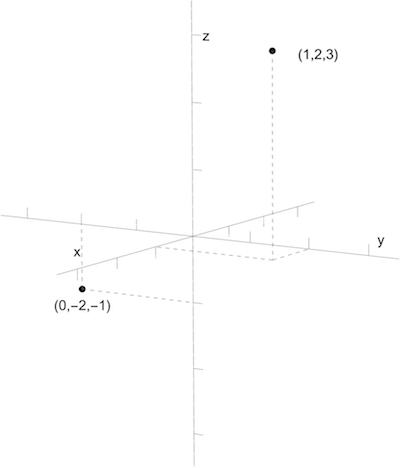
Points plotted in 3D

3-Dimensional Vector Addition

Points in three-dimensional space can also be considered as vectors, just as we did in two dimensions. Instead of considering the point \((x,y,z)\) as just a point, we visualize it as an arrow starting at the origin \((0,0,0)\) and pointing to the point \((x,y,z)\). The is pictured below, where we consider the same points graphed above as vectors.

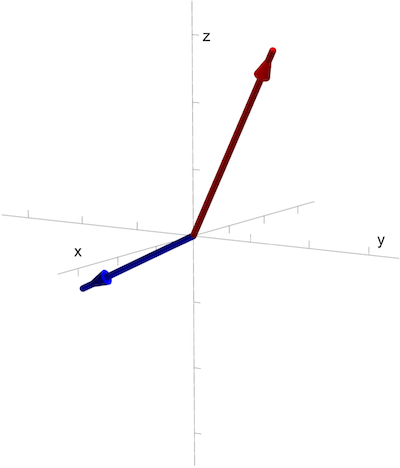
Vectors plotted in 3D

The vector addition operation we discussed in two dimensions also generalizes naturally to three-dimensions. There's an intuitive way to add elements of \(\mathbb{R}^3\), by just adding the corresponding elements in the ordered triples:

For the two points we've considered above, we have

This operation also has the same geometric meaning - if we consider the ordered triples as vectors, then addition corresponds to moving one arrow to begin at the end of the other, then drawing a new vector to the end of that arrow. This is clearer in pictures, shown below. The red vector is \((1,2,3)\), the blue vector is \((0,-2,-1)\) and the sum \((1,0,2)\) is shown in black. The translates of the vectors are also shown to demonstrate that the parallelogram rule similarly applies in 3-dimensions.

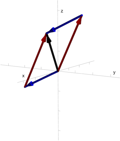
Vector addition in 3D

This addition operation generalizes naturally to all higher dimensions - we can always add two element of \(\mathbb{R}^k\) by considering those elements as ordered \(k\)-tuples of numbers and just adding the corresponding numbers. (In four dimensions, this exactly gives the operation of addition of quaternions, but we'll discuss this more later.) This becomes difficult, if not impossible, to visualize in higher dimensions, though. The set \(\mathbb{R}^k\), along with this vector addition operation, is the main example of a vector space, an extremely important concept in geometry that we'll discuss in more depth in a later post.

We see that the set of \(\mathbb{R}^3\) of triples of real numbers can be given an addition operation, and an inverse subtraction operation is also easy to define: we just subtract the corresponding elements in the triples. Taking a different set of vectors to subtract, if we have the vectors \(v_1 = (-1,1,3)\) and \(v_2 = (1,2,2)\), then the subtraction \(v_1 - v_2\) results in the vector

This also has an easy interpretation in terms of vectors - subtracting a vector is the same as adding a vector pointing in the opposite direction. This is illustrated below:

Vector subtraction in 3D

In these images, the red vector is \(v_1\), the blue vector is \(v_2\), and the black vector corresponds to the subtraction \(v_1 - v_2\), which we'll call \(v_3\). The green vector is the vector \(-v_2 = (-1,-2,-2)\), the vector with the same magnitude as \(v_2\) but pointing in the opposite direction. Note that the subtraction \(v_1 - v_2\) is the same as the vector addition \(v_1 + (-v_2)\), as illustrated in the left figure.

The image on the right gives another way to interpret the subtraction. We have that \(v_1 - v_2 = v_3\), which we can rearrange to say that \(v_1 = v_3 + v_2\), which is the vector addition shown on the right.

What About Multiplication and Division?

Recall that all our work so far has been to try to understand number systems that have addition, subtraction, multiplication, and division operations. We've done half of that work in \(\mathbb{R}^3\) by defining a way to add and subtract triples of real numbers, and this operation corresponds geometrically to vector addition and subtraction. What happens when we try to define multiplication and division operations?

As mentioned earlier, it turns out this is impossible - one has to increase to four dimensions and consider the quaternions in order to be able to define a higher-dimensional number system that has a valid multiplication and division operation. Proving exactly why such an operation can't exist in three dimensions will have to wait for a later post, but in order to understand this impossibility it's worth it to try to see what happens when we attempt to make such a definition.

In particular, we could try to make the most obvious definition for multiplication - what if we just multiply two triples by multiplying their corresponding entries? That is, we can define a multiplication operation by

This certainly defines some kind of operation, but the problem is that there is no way to define a corresponding inverse or division operation for this multiplication. To see why, consider the multiplication below:

Call the two vectors that we've defined \(v_1\) and \(v_2\), and let \(\mathbf{0}\) denote the vector that consists of all zeros, so that we can write the above in a shorter form as \(v_1 \cdot v_2 = \mathbf{0}\).

We'd like to define an inverse for \(v_2\), which we would denote by \(v_2^{-1}\), such that multiplication by \(v_2^{-1}\) undoes multiplication by \(v_2\). If we could do that, then we'd be able to write

and since \(v_2^{-1}\) undoes multiplication by \(v_2\) we'd end up with the expression

But this can't possibly be true - no matter what the vector \(v_2^{-1}\) is, it's clear that multiplying it by \(\mathbf{0}\) will always result in \(\mathbf{0}\), and \(v_1\) and \(\mathbf{0}\) are not the same thing. There's simply no way to define a vector \(v_2^{-1}\) that will undo multiplication by \(v_2\) using this definition of a multiplication operation.

There is a more general terminology for this phenomenon - if a set has an multiplication operation and it's possible to multiply two non-zero objects together and obtain zero, then the multiplication is said to have zero divisors. And the same argument above applies in general - if a multiplication operation has zero-divisors, it's not possible to define an inverse operation that defines division. With a bit more advanced math (that we might see in a later post), one can show that any multiplication operation on \(\mathbb{R}^3\) has to have zero divisors, and so it is impossible to define a multiplication operation on \(\mathbb{R}^3\) that also has a corresponding division operation.

Next Time: Vector Products in Three Dimensions

This is not to say that there are no useful concepts of "multiplication" or "product" in three dimensions. In fact, there are two, and they may be familiar to those who have learned either physics. They are the dot product and the cross product, named for the symbols used to write them. Of course, these operations don't have a corresponding division operation, but that doesn't mean they can't still be useful.

In the next posts, we'll learn what these products are and see why they're important to geometry in three dimensions. These products will also provide the crucial link between the three-dimensional geometry we have been discussing and the 4-dimensional geometry of the quaternions.