Implementing the Binomial Option Pricing Model
Posted on Thu 15 March 2018 in Finance
In the previous posts in this series, we've described a model for stock price movements that can be used to find prices of simple European call and put options. The model works by dividing the life of the option into some number of discrete intervals, and assuming that the stock price randomly moves either up or down by a fixed percentage over each short interval. This gives a tree of possible prices for the stock, and the option's value at each node in this tree can be computed as a discounted expected value of the future value of the option at later nodes in the tree, where the expected value is computed using risk-neutral probability and the discount factor is determined by the risk-free interest rate.
In those previous posts, we computed prices given by this model in very simple cases, with only one or two steps. For the model to be effective, a larger number of steps will be required, and so it will no longer be feasible to compute by hand as we've done before. In this post, we'll see how to implement the model in Python, consider a better way for choosing the parameters \(u\) and \(d\) in the model, and then discuss the rate of convergence of the algorithm
The First Implementation
We begin by giving a first, direct implementation of the model to compute the price of a call option.
import math

def first_binomial_call(S, K, T, r, u, d, N):
    dt = T/N
    p = (math.exp(r * dt) - d)/(u - d)
    C = {}
    for m in range(0, N+1):
            C[(N, m)] = max(S * (u ** (m)) * (d ** (N-m)) - K, 0)
    for k in range(N-1, -1, -1):
        for m in range(0,k+1):
            C[(k, m)] = math.exp(-r * dt) * (p * C[(k+1, m+1)] + (1-p) * C[(k+1, m)])
    return C[(0,0)]
The notation in this implementation is essentially identical to the notation we used to describe the model in the previous post. We use all of the same symbols to denote the parameters in the model, except we write dt instead of \(\Delta t\) for the length of the time interval of each step. We use a dictionary to store the values of the option at each node, and use the same notation for the keys of the dictionary, that is, C[(k,m)] above is the same as the value \(C(k,m)\) in the previous post, meaning the value of the option at the node that is \(k\) steps into the tree, with \(m\) of those steps being up movements in the stock.
The implementation above proceeds by computing the value of the time step dt and finding the risk-neutral probability p. The first loop then finds the value of the option at the end of the tree, using the normal payoff of a call option (the stock price minus the strike price if that is positive, and otherwise 0). The next pair of nested loops then works backward through the tree to iteratively fill in the value of the option at every node. The value at the root node is returned as the price of the option today.
We can do a very simple check of our implementation to make sure that it can reproduce the computation that we've already done by hand. In the first post in this series, we priced a call option on a stock that is worth $100 today and is assumed to be worth either $120 or $80 in three months time. We ignored interest rates in that model and only used one step. If the strike price on the option is $100, then our implementation of the model gives that the price is
first_binomial_call(100, 100, 1, 0, 1.2, 0.8, 1)
10.0
the same price we computed before by hand. At least our implementation appears correct in this simple case!
Now that we have a computer to do the work for us, we can run the model with many more steps, that is, we can increase the value of \(N\) to find a better price for the option. There is one subtlety with our implementation, though, that makes this difficult. To understand the problem, we can see what happens as we increase the number of steps.
for N in [1,10,100,200,300,400,500]:
    print("With N = {:3d}, the price is {:.2f}".format(N,first_binomial_call(100, 100, 1, 0, 1.2, 0.8, N)))
With N =   1, the price is 10.00
With N =  10, the price is 25.62
With N = 100, the price is 68.55
With N = 200, the price is 84.56
With N = 300, the price is 91.90
With N = 400, the price is 95.61
With N = 500, the price is 97.58
As the number of steps increases, the price is going up, and quite drastically, to approach the current value of the stock. This doesn't make sense - the price of the option should not be the same as the price of the stock. What's going on here?
The problem concerns our choice of \(u\) and \(d\) - these values represent the change in price of the stock option over each small time interval. As such, the value of \(u\) and \(d\) depend implicitly on the length of that time interval. Therefore if we increase the number steps in the model, thus decreasing the length of each interval, but leave \(u\) and \(d\) constant, we're actually changing the total amount we're allowing the stock price to move. In our specific example, with one step we have that the final value of the stock is either \(Su = 100 (1.2) = 120\) or \(Sd = 100(0.8) = 80\), that is, the stock price can move by 20% every three months. If we increase \(N\) to 3 without changing \(u\) and \(d\), then we have that stock price can change by 20% every month, and the final values of the stock can range between \(Su^3 = 100(1.2)^3 = 172.80\) and \(Sd^3 = 100(0.8)^3 = 51.20\), which is a very different range. Therefore, as we change \(N\), we need to modify \(u\) and \(d\) as well to keep our predictions about the future movement of the stock price consistent. This leads us to consider how best to determine the value of \(u\) and \(d\) in our model.
Choosing \(u\) and \(d\): Volatility
Our values of \(u\) and \(d\) represent the possible return on the stock over a short period of time. As such, a large value of \(u\) (or a small value of \(d\)) means that the price of the stock could change drastically over a short period of time. A stock price that changes drastically over a period of time is called volatile, and so \(u\) and \(d\) in some sense describe the volatility of the stock. It's really the volatility that we'd like to have as the parameter in the model. That is, instead of choosing \(u, d\) as independent parameters in our model, as we've done so far, we're going to compute \(u\) and \(d\) from the values of \(T\) and \(N\) along with a third number that measures volatility. This will solve the problem we have above by making explicit the dependence of \(u, d\) on the variable \(dt\).
Volatility, in this setting, is really just another word for risk. If a stock price was not volatile, that would mean it didn't move, or moved absolutely predictably, and would not be risky. A more volatile stock, that is, one that can change wildly in price, is clearly more risky than an asset with a price that can only change by a small amount.
There's already a mathematical way to describe volatility or riskiness, called standard deviation. If \(X\) is a random variable, with expected value \(E(X)\), also called the mean and denoted by \(\mu\), then the variance, denoted by \(\sigma^2\), is defined to be \(\sigma^2 = E((X-\mu)^2)\), that is, the variance is the expected value of the square of the difference between an observed value of the random variable and the mean. The standard deviation, \(\sigma\), is the square root of the variance - knowing one determines the other. If a random variable has a large standard deviation, that means that a wider range of values around the mean are likely, while a small standard deviation means that the variable is more likely to be observed to be close to its mean. Put another way, if we tried to guess the value of the random variable by guessing the mean, then the standard deviation gives a way to measure the likely error of such a guess.
In our model, we will assume that the return on the price of the stock underlying the option is a random variable with a fixed variance of \(\sigma^2\). This variance will be independent of time in the sense that, if \(S\) is the price of the stock today and \(S^\prime\) denotes the stock price after \(\Delta t\) units of time, considered as a random variable, then we will assume that the variance of the random variable \(\frac{S^\prime - S}{S}\), the return on the stock, will be \(\sigma^2 \Delta t\). For example, if we measure time in years, then choosing \(\sigma = 0.2\) would say that the standard deviation in the returns on the stock is assumed to be 20% over the year, or \(0.2(\sqrt{0.5}) = 14.1\%\) over 6 months, etc. (For the reader familiar with statistics, we're ultimately assuming that the returns on the stock price over a time period of \(\Delta t\) are normally distributed with variance \(\sigma^2 \Delta t\). The mean of the normal this distribution is chosen so that the expected value of the stock at any particular time grows according to the risk-free rate - this is essentially done using our formula for \(p\), the risk-neutral probability, and so we won't worry about it here.)
Based on this value of \(\sigma^2\), we'll choose \(u\) and \(d\) as follows:
A full explanation of why we make these choices will have to wait for a later post. The short answer is that these choices mean that our model will be a good approximation for a popular model of stock prices called geometric Brownian motion. For now, we'll just make use of this choice and make note of a two properties of our choices. First, the larger \(\sigma\) is, the larger \(u\) is, hence the smaller \(d\) is, and therefore the greater the spread of values in our model, matching with the intuition we developed earlier. Second, the fact that \(ud = 1\) will allow us to simplify some computations.
The Final Model
With this method for choosing \(u\) and \(d\) in our model, we can make an easy modification to the first implementation above to give the following model. Note that the parameters u and d have been replaced with vol, the volatitlity of the stock. We use vol in our code instead of the Greek letter \(\sigma\).
def binomial_call(S, K, T, r, vol, N):
    """
    Implements the binomial option pricing model to price a European call option on a stock
    S - stock price today
    K - strike price of the option
    T - time until expiry of the option
    r - risk-free interest rate
    vol - the volatility of the stock
    N - number of steps in the model
    """
    dt = T/N
    u =  math.exp(vol * math.sqrt(dt))
    d = 1/u
    p = (math.exp(r * dt) - d)/(u - d)
    C = {}
    for m in range(0, N+1):
            C[(N, m)] = max(S * (u ** (2*m - N)) - K, 0)
    for k in range(N-1, -1, -1):
        for m in range(0,k+1):
            C[(k, m)] = math.exp(-r * dt) * (p * C[(k+1, m+1)] + (1-p) * C[(k+1, m)])
    return C[(0,0)]
There are only two changes here from the implementation above. First, our model now computes u and d from vol. Second, we used the fact that \(d = 1/u = u^{-1}\) to write
simplifying our computation of the final price of the stock.
Let's see how this implementation performs with the previous example we computed by hand. We won't be able to exactly replicate that example, since before we had chosen \(u = 1.2\) and \(d = 0.8\), and therefore we don't have that \(ud = 1\). Instead, we'll choose the volatility to match \(u\), which we can see is done by choosing vol \(= \log(1.2)\). Then, finding prices for various values of \(N\), we have:
for N in [1,2,10,100,200,300,400,500]:
    print("With {:3d} steps, the price is {:.2f}".format(N,binomial_call(100, 100, 1, 0, math.log(1.2), N)))
With   1 steps, the price is 9.09
With   2 steps, the price is 6.44
With  10 steps, the price is 7.08
With 100 steps, the price is 7.25
With 200 steps, the price is 7.25
With 300 steps, the price is 7.26
With 400 steps, the price is 7.26
With 500 steps, the price is 7.26
We've fixed the issue from before - now, the values of \(u\) and \(d\) are recomputed as we change \(N\). As \(N\) increases, we see that the price given by the model converges fairly quickly to the value of $7.26, which we will take to be a fair price for the option.
Analyzing the Performance
To end this post, we'd like to understand how well our algorithm performs, and specifically how quickly it converges on a particular value. That is, we've seen that increasing \(N\) increases the accuracy of the price, so how large does \(N\) need to be to ensure that we've found a good price? If getting an accurate price requires using millions of steps and therefore requires a long computation time, the algorithm will be useless. Another difficulty is that this question of the rate of convergence assumes that the algorithm does in fact actually converge to some value. Put mathematically, if we fix all of the parameters in our model except \(N\) and let \(f(N)\) denote the output of the algorithm for a particular number of steps, does \(\displaystyle\lim_{N \rightarrow \infty} f(N)\) exist?
The answer, in this particular case, is yes. If fact, with some more sophisticated mathematics one can show that this limit always exists, and that in fact there is a relatively simple formula that allows us to compute the value of any European call (or put) option from the parameters \(S, K, T, r,\) and \(\sigma\). This formula is known as the Black-Scholes formula. We won't give the exact formula in this post, but it's simple enough that it can be computed essentially instantaneously by a computer, while our model will take a perhaps a second or two to run with \(N = 1000\) steps on a basic laptop.
So why have we done all of this work with the binomial model when there's an arguably simpler and faster formula for the option price? There are two main reasons:
-
This binomial model is one method to derive the Black-Scholes formula. As stated above, the Black-Scholes formula is essentially the limit of our our model as \(N \rightarrow \infty\). This isn't the original way that this formula was derived, but this method requires less advanced mathematics than other methods. The derivation through the binomial method uses no math more difficult than standard probability theory, while other methods involve more difficult techniques like stochastic calculus.
-
The binomial model can be used in situations where a simple "limit" formula doesn't exist. For example, we've so far only dealt with European options, which can only be exercised at one particular time. By contrast, American options give the right to exercise the option at any time before expiry, and the possiblity of early exercise makes them more difficult to price. Depending on the exact nature of the American option, it is not always possible to find a Black-Scholes style formula, and the only way to price the option is using a numerical approximation like our binomial model. We'll explore this more in the next post.
So, even though we have a quick formula to give us the "correct" answer, it's instructive to see how well our binomial method works to find that answer. In particular, how large does \(N\) need to be in order for the model price to match the Black-Scholes price?
We investigate this in the chart below. In the chart, we use our model to find a price for a European call option with \(S = 100\), \(K = 120\), \(T = 1\) year, \(r = 1\%\), and \(\sigma = 0.2\). These values were chosen arbitrarily. The number of steps used in the model is on the \(x\)-axis. The price is plotted on the \(y\)-axis. The red horizontal line is the price for the option given by the Black-Scholes formula - in this case, $2.34. The dotted horizontal lines are at 2.335 and 2.345, so that any value between those lines would agree with the Black-Scholes price to the nearest cent.
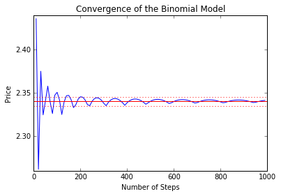
We can see that, in this particular case, our model converges fairly quickly - it only takes around 200 steps for the model price to be accurate within rounding error. Note that our option has an expiration time of 1 year, and there are roughly 250 trading days in a year, so our model is fairly accurate if we take the step size to be about one trading day.
Next time - Beyond European Calls
We now have a workable model to give prices for European call options on stocks, and a straightforward and fairly efficient implementation of the model in Python. Next time, we'll finish our discussion of this method by seeing how to modify our implementation to find prices for other type of options, including the American options discussed above.