The Binomial Options Pricing Model

Posted on Fri 02 March 2018 in Finance

In the previous post introducing the Binomial Options Pricing Model, we discussed a very simple model for the movement of stock prices. In that model, we assumed that at the end of a certain period of time, the value of a stock could take on one of two possible values. We then used a variety of arguments, including replication and risk-neutral pricing, to determine a price for a call option on the stock.

In this post, we'll see how this model can be improved to predict the movement of stock prices more accurately. We'll also make some simple modifications that allow us to consider some of the complicating factors we ignored in the last post, like interest rates.

The Two-Step Model

Let's return to the example from the previous post, in which we assumed that a stock worth $100 today would be worth either $80 or $120 in six months' time. We used this assumption to find a price for a call option on the stock, expiring at the end of the same six-month period with a strike price of $100.

This model essentially assumed that there would be only one movement in the stock price in 6 months, or put another way, that we would only observe the stock price once over the life of the option. What if we looked multiple times?

In particular, instead of assuming that the stock could either increase or decrease by $20 over a six-month period, let's assume that the stock can either increase or decrease by $10 over each three-month period. There are now four different possibilities for how the stock price can change as over the six-month period - it can either move up twice, move up and then down, move down and then up, or move down twice. Letting $u, d$ denote up and down movements, respectively, and using $S$ to denote the stock price today, $S_{u}$ to denote the price after an up movement, $S_{du}$ denote the price after a down and then an up movement, etc., we're left with the following tree of possible prices for the stock.

Two-Step Binomial Tree

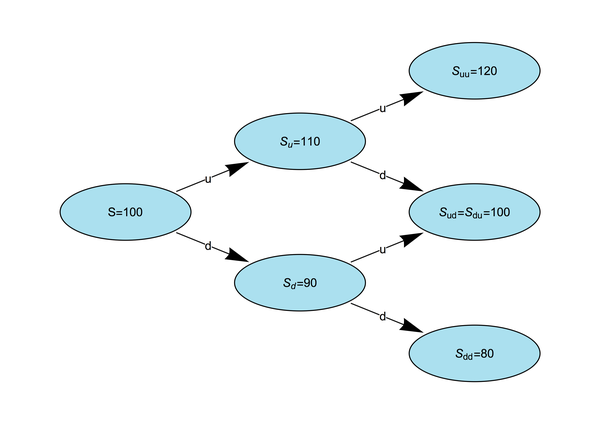
It's important to note that the price after an up movement in the first period followed by a down movement in the second period is the same as the price after a down movement followed by an up movement. This will simplify the computations, especially when we fully generalize the model to include many intermediate steps. The order of the up and down movements does not matter, only the total number of up movements and the total number down movements.

How do we find a price for the option under this new model? The method is to view this larger tree as a collection of smaller one-step models and repeatedly apply the pricing methods we described in the last post. In particular, we can zoom in on just one part of the tree, the portion consisting of $S_u$ and the branches to $S_{uu}$ and $S_{ud}$. If the final price is $S_{uu} = 120$, then the option will be worth $20, and if the final price is $S_{ud} = 100$, then the option will be worth $0. We can then find the value of the option in three months time, assuming that the stock increased over the first period. The easiest method for this is to use risk-neutral pricing. We can compute that the risk-neutral probability in this situation is $p = 1/2$ (just as it was in the last post), and therefore the value of the option at the $S_u$ node of the tree is

\begin{equation*} C_u = 20 (1/2) + 0 (1/2) = 10 \end{equation*}

We can repeat this computation to find the value of the option at the $S_d$ node in the tree, that is, the value of the option in three month's time under the assumption that the stock first moves down. From an initial value of $S_d = 90$, the stock price can either move to $S_{dd} = 80$ or $S_{du} = 100$. In either case, the option will be worthless in six months (the strike price is 100), and therefore the value of the option at the $S_d$ node is zero.

Finally, if we know that the values $C_u = 10$ and $C_d = 0$ for the option at the $S_u$ and $S_d$ nodes, then we can work backwards to find the initial value of the option. The risk-neutral probability will once again be $p = 1/2$, and so the value of the option today is

\begin{equation*} C = 10 \times (1/2) + 0 \times (1/2) = 5 \end{equation*}

The tree with the value of the option at the various nodes is shown below.

Option Values in Two-Step Binomial Tree

This value is different from the value of $10 we found in the last post, but it's not hard to see why. In the one-step model, we only had two possible values for the stock price at expiry, one in which the option has value (an up movement) and one in which it does not (a down movement). In the two step model, we have assumed that there are more possible values for the final price of the stock, and the option is worthless for these new possible values. Thus under the new model there will be fewer opportunities to exercise the option and gain value from it, and so the option is worth less in the new model.

It's clear from the above example how we could continue to improve the model - instead of dividing the six-month time period into two three-month periods, we could divide it into 3, 4, 5, or even more periods. Perhaps we could divide the interval into 20 periods, and the price could move up or down by one dollar in each period. This would still imply that the stock price at the end of six months has a value between $80 or $120, but in this case any dollar value between these two numbers is also a possible outcome in the model, which is a much more realistic model than the two or three values we've had in the examples so far. Before discussing this generalization, though, we will consider how interest rates affect the model.

Adding Interest Rates

So far, we've ignored how interest rates and the time value of money would change our computations. For example, in computing the value $C_u$ above, we assumed that if the option was expected to be worth $10 at the end of the six-month period, its value at three months should be the same. This is not the case, though, as the value of $10 today is more than the value of $10 in three month's time. After all, if an investor has $10 today, they could always a put the money into a completely safe investment, perhaps something like a savings account, and earn a small amount of interest so that, after three months time they have $10.01 instead of just $10.

The value of a payment therefore depends not only on the actual dollar amount of the payment, but on when the payment is made. To be consistent in finding prices for financial assets, we need a way to find the value today of a payment made in the future, so that all prices under consideration are always in "today's" dollars. The idea is that if one will receive $$Y$ in $T$ month's time, the value of that payment today is the amount of money that would have to be invested today in a risk-free investment so that in $T$ months that safe investment will have grown to $Y$.

Risk-free investments do not actually exist in truth, but mathematical finance generally assumes that such investments are available. This is because short-term bonds issued by stable governments in their own currency are very safe investments. There is of course the possibility that, say, the US government may default on its debt, but this would have such major economic effects that accurately pricing options would be the least of an investor's worries. Still, because these assets have no risk, the rate of return is small - the current yield on three-month treasury bills is around 1.5% annually. The rate of return of the risk-free investment is appropriately known as the risk-free rate.

To simplify computations, we'll assume that all interest is compounded continuously. That is, if $r$ is the risk-free interest rate, written as a decimal (so that 1.5% = 0.015), then if one invests $P$ dollars for a period of $t$ years, the investment will grow to $Pe^{rt}$, where $e = 2.71828\ldots$ is Euler's number, the base of the natural logarithm. On the other hand, a cash payment of $X$ dollars at some time $t$ years in the future will have a present value today of $Xe^{-rt}$. We'll use this present value formula in the next section to compute the value of an option today if its future expected value is known. The number $e^{-rt}$ is called a discount factor, since it is used to discount future values of a cash flow to their smaller present values.

Note that the risk-free interest rate, and the related discount factor, are only appropriate for finding the present value of risk-free assets. In general, if we wanted to find the present value of a future payment that had some amount of uncertainty, we'd need to choose an interest rate that reflected the uncertainty. We could think of this as the rate of return that could be expected from investing our money in an equally risky asset. The expected values of the options we are pricing are technically risky, so in principle we should be finding a discount factor that reflects those risks. This represents one more advantage of risk-neutral pricing - we can avoid the work of having to decide on a discount factor that is appropriate to the risk of the option. Instead, we ignore the risk, as we've done before, and use the risk-free interest rate to simplify our computations.

The Many-Step Model

With interest rates figured out, we're now ready to give the actual model. There's just one final change to make. In our two-step example above, we've assumed that the stock price moves by adding or subtracting fixed amounts. In our final model, we'll instead assume that the price moves by a fixed percentage in each period. This turns out to more accurately model the movement of stock prices, as we'll discuss in a later post.

We'll also abandon the numbers we used in our specific examples and replace them with variables. Let $S$ denote the price of the stock today, and let $T$ denote the time until expiry of the option, in years. We'll divide this period into $N$ equal time intervals, of length $\Delta T = T / N$. Finally, assume that in each time period, the stock price changes by either multiplying by $u$, which we consider as an up movement, or by $d$, the down movement. For example, if we assume that a stock can grow by 2% over a short time interval, then we pick $u = 1.02$. Thus after one period, the stock will have a value of either $Su$ or $Sd$. We need to assume $d < e^{r\Delta T} < u$, where $r$ is the risk-free interest rate, to avoid the possibility of arbitrage.

We can then consider a tree of possible prices for the stock. If $k$ time periods have passed, then the stock price at that time is determined by the number of up and down movements in the stock. Since the order of the stock movements does not matter, we have that if $k$ time periods have passed and the stock price has increased over $m$ of those periods (and therefore decreased over $k-m$ of those periods), the price of the stock at that time is

\begin{equation*} S(k,m) = Su^{m}d^{k-m} \end{equation*}

This explains why this model is known as the binomial model - the price of the stock could be determined by flipping a coin $k$ times and assuming that the stock moves up each time a head appears. More properly, we should consider a weighted coin that has a probability $p$ of coming up heads. The so-called "binomial distribution" is the distribution in probability used to model coin flips.

We can now use the tree of stock prices produced by this formula to find the value of the option. Assume we're pricing a call option with strike price $K$. We can easily find the value of the option at the expiry in each of the possible nodes of the tree. Under our model, the price of the stock has $N+1$ possible values at expiry, depending on the number of up-movements in the stock. For each of these possible stock prices, the option is worth

\begin{equation*} C(N,m) = \max(S(N,m) - K, 0) \end{equation*}

(Here $m$ can be any of the values $m = 0,1, \ldots, N$). Interpreting the above formula, the option is worth the difference between the price of the stock and the strike price if the stock is worth more than the strike, and zero otherwise (the case in which the option is not exercised).

Once we know the value of the option at the end of the tree, we can work backward as before to figure out the value of the option at every node. Let $C(k,m)$ denote the value of the option at the node that is $k$ steps into the tree with $m$ up movements in the stock price. The two following nodes in the tree are $C(k+1,m+1)$ (if the price moves up) and $C(k+1,m)$ (if the price moves down). If we let $p$ denote the risk-neutral probability of a movement up, then the expected value of the option in the next step is

\begin{equation*} p C(k+1,m+1) + (1-p) C(k+1,m) \end{equation*}

and so the value of the option at $C(k,m)$ is the above expected value, discounted to today using the risk-free interest rate. That is

\begin{equation*} C(k,m) = e^{-r \Delta T} \left( p C(k+1,m+1) + (1-p) C(k+1,m) \right) \end{equation*}

With this formula, we can work our way backward through the tree until we can compute the value $C(0,0)$, which is the value of the option today, and therefore the price.

Finally, we need to find the value of the risk-neutral probability. From our discussion in the last section, it should be chosen so that the stock price at any node in the tree is equal to the expected value of the stock price in the child nodes, appropriately discounted. That is, we need to chose the $p$ such that the following formula is satisfied:

\begin{equation*} S(k,m) = e^{-r \Delta T} \left( p S(k+1,m+1) + (1-p) S(k+1,m) \right) \end{equation*}

Using the formula $S(k,m) = Su^{m}d^{k-m}$, we can solve this equation to find that the risk-neutral probability is

\begin{equation*} p = \frac{e^{r \Delta T} - d}{u-d} \end{equation*}

Note that this formula does not depend on the values of $k$ and $m$, so that the risk-neutral probability is the same everywhere in the tree. In contrast, we could consider using the replication method discussed in the previous post to compute the value of the option at each node. If we tried this, however, we'd notice that in general the payoffs at the child nodes are different as we move through the tree. Therefore we'd have to find a different replicating portfolio for every node, which would be a lot more work. Using risk-neutral pricing allows us to avoid these unnecessary computations and greatly simplifies the model.

Summarizing the Model

And that's it! After a good deal of work, we've found a model that can be used to find the price of a European call option on a stock. The model is as follows:

Divide time until expiry of the option into $N$ intervals. On each interval, assume that the stock can move up or down by a factor of $u$ or $d$, respectively.
This assumption generates a tree of possible prices for the stock. At the leaves of the tree, we can find the value of the option for the given stock price represented by that node by using the payoff determined by the option contract.
Working back through the tree, we can find the value of the option at any node as long as we know the value of the option at the two child nodes. We do this by finding the expected value of the option at those two child nodes using the risk-neutral probability, then discounting that value using the risk-free interest rate.
This process continues until the value of the option at the root node, representing the value today, is found, which is the price of the option.

The model uses three properties of the option that are known, namely the stock price today, the strike price of the option, and the time until expiry. It also takes as input the value $r$ for the risk-free interest rate available in the market. The model also has three "tuning parameters" that we can choose ourselves, namely the size of the movements $u$ and $d$ and the number of steps in the tree $N$. If we want our model to be useful, we still need to decide how to choose these parameters.

As we saw above, our model is more accurate the more steps we include. Of course increasing $N$ increases the number of nodes in our tree, and so larger values of $N$ will take longer to compute. Therefore, we should choose $N$ as large as possible while still making sure that our algorithm is computationally feasible. We'll discuss this more in the next post, when we actually implement this model in Python and analyze its performance.

Choosing $u$ and $d$ is more difficult. There are good techniques for choosing these values, but understanding them requires making some more explicit assumptions about the movement of stock prices which we'll discuss in a later post. For now, it's enough to say that choosing $u$ and $d$ amounts to forecasting the future movement of the stock. We'll therefore choose them somewhat arbitrarily, picking feasible values and tweaking them as necessary so that the range of possible stock prices in the model accords with whatever prediction about the future movement of the stock we wish to make.

Next Time - Implementing the Model

Now that we've found a model we can use, it's time to actually put it into practice. In the next post, we'll implement this model in Python and run it on a few simple examples. We'll also analyze its performance, and see how our implementation can be used to price other types of options as well.